From Equations to Code: Training a Laplace Neural Network
In the first post we introduced a Laplace neuron (an LTI block + optional static nonlinearity) as a dynamical building block. In the second post we showed how to compute gradients through a small Laplace Neural Network, not through time, but through the network graph, yielding closed-form gradients in the Laplace domain.
Today we'll put the theory to work, make a clean, runnable Python implementation that learns a simple physical system from data and even generalize to inputs it never saw.
We are going to:
- build an actual Laplace Neural Network as a directed acyclic graph (DAG) of Laplace neurons,
- train it end-to-end on a simple physical system,
- compare it to RNN baseline ,
- test its extrapolation capabilities on input signals outside of training distribution.
The setup: identify a mass–spring–damper
If the world is a hierarchy of dynamical systems, the mass–spring–damper is the “hello, world” of that hierarchy. Three parameters, one second order differential equation, and an entire spectrum of behaviors, settling, overshoot, emerging from a tiny polynomial in \(s\) domain.
We’ll work with a standard second order plant:
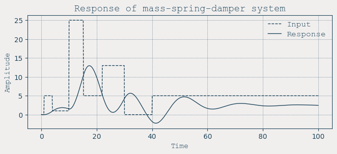
and drive it with a piecewise constant input \(u(t)\). The system response is the position \(y(t)\). Our goal is system identification or to learn a network \(f_0\) such that \(f_0[u(t)] \approx y(t)\), where \(y\) is the plant's position response.
# System parameters
m, c, k = 20, 3, 2
t = np.linspace(0, 100, 1000)

# Arbitrary piecewise constant input
u = np.zeros_like(t)
u[10:] = 5
u[40:] = 1
u[100:] = 25
u[152:] = 5
u[220:] = 13
u[300:] = 0
u[400:] = 5

# System response
plant = signal.TransferFunction([1], [m, c, k])
_, position, _ = signal.lsim(plant, U=u, T=t)

The model: Laplace Neural Network
Each node of the network \(j\) is a Laplace neuron that has:
- an input \(u_j(t)\) formed by weighted sum of parent outputs,
- a linear time-invariant block \(H_j\) (its transfer function),
- optionally a static nonlinearity \(\phi\) before the LTI block.
For this experiment we set \(\phi\) to the identity, so each node reduces to pure LTI block. Swapping in a nonlinearity (e.g. \(\delta\)ReLU from the first post) is plug-and-play, the only change in the gradients is a local \(\phi'\) factor to the sensitivities (see next section).
Each Node carries a transfer function \(H_j(s)\) and the transfer functions of its parameter derivatives \(\partial H_j / \partial \theta\). The network is a feed-forward DAG (the same 1–3–3–1 layout we used before): three neurons read the external input, three combine them, and one produces the output.
@dataclass
class Node:
    name: str
    params: Dict[str, float] = field(default_factory=dict)
    build_tf: Callable[[Dict[str, float]], signal.TransferFunction] = lambda p: tf_one()
    build_param_derivs: Callable[[Dict[str, float]], Dict[str, signal.TransferFunction]] = lambda p: {}
    tf: signal.TransferFunction = field(init=False)               # H_j
    d_tf: Dict[str, signal.TransferFunction] = field(init=False)  # {∂H_j/∂θ}

    def __post_init__(self):
        self.rebuild()

    def rebuild(self):
        self.tf = self.build_tf(self.params)             # H_j
        self.d_tf = self.build_param_derivs(self.params) # {∂H_j/∂θ}
Concrete builders functions
For concreteness I instantiate a lightweight first-order family,
and supply analytical transfer function derivatives \(\partial H / \partial k,\ \partial H / \partial \tau,\ \partial H / \partial \zeta\).
def first_order_tf_builder(p):
    return signal.TransferFunction([p["k"]], [p["tau"], p["zeta"]])

def first_order_tf_derivs(p):
    k, tau, zeta = p["k"], p["tau"], p["zeta"]
    dH_dk    = signal.TransferFunction([1.0],           [tau, zeta])                    # ∂H/∂k
    dH_dtau  = signal.TransferFunction([-k, 0.0],       [tau**2, 2*tau*zeta, zeta**2])  # ∂H/∂τ
    dH_dzeta = signal.TransferFunction([-k],            [tau**2, 2*tau*zeta, zeta**2])  # ∂H/∂ζ
    return {"k": dH_dk, "tau": dH_dtau, "zeta": dH_dzeta}
Transfer function algebra helpers
We'll manipulate TFs symbolically and then simulate their responses with scipy.signal.lsim. These helpers mirror block diagram operations.
def tf_series(a, b):     # Series: b ∘ a
    num = np.polymul(a.num, b.num)    # Multiply numerators
    den = np.polymul(a.den, b.den)    # Multiply denominators
    return signal.TransferFunction(num, den)

def tf_add(a, b):        # Parallel sum: a + b
    num = np.polyadd(np.polymul(a.num, b.den), np.polymul(b.num, a.den))
    den = np.polymul(a.den, b.den)
    return signal.TransferFunction(num, den)

def tf_gain(g):          # Scalar gain as TF
    return signal.TransferFunction([g], [1.0])

def tf_zero(): return signal.TransferFunction([0.0], [1.0])
def tf_one():  return signal.TransferFunction([1.0], [1.0])
tf_seriescomposes two blocks as a serial connection.tf_addadds two branches in parallel.tf_gainis a static edge weight as a TF.tf_zero/oneare identities for sums/series.
The network as Directed Acyclic Graph
We wire nodes as a directed, weighted graph and insist on topological order so signal flow is left to right exactly once. No hidden loops, no implicit recurrences, just a clean acyclic pass where each node \(j\) collects its weighted parents outputs, applies its dynamical response and hands the result downstream.
@dataclass
class Edge:
    src: Union[int, str]   # node id or "src:*"
    dst: int
    w: float               # trainable edge weight
@dataclass
class LTINetwork:
    nodes: List[Node]
    edges: List[Edge]
    output_node: int
    sources: Dict[str, np.ndarray]  # time-series inputs (e.g., {"src:u": u})
    t: np.ndarray

    # caches from the last forward pass
    u: Dict[int, np.ndarray] = field(init=False, default_factory=dict)  # inputs to nodes
    x: Dict[int, np.ndarray] = field(init=False, default_factory=dict)  # outputs of nodes
    topo: List[int]          = field(init=False, default_factory=list)

    def __post_init__(self):
        self._check_dag_and_build_topo()
Topological order via Kahn’s algorithm ensures parents come before children.
Forward pass: simulate, don’t unroll
Instead of unrolling a recurrent state, we simulate each neuron’s transfer function once per batch with scipy.signal.lsim:
def forward(self) -> np.ndarray:
    self.u = {j: np.zeros_like(self.t) for j in range(len(self.nodes))}
    self.x = {}
    parents_by_dst = defaultdict(list)
    for e in self.edges:
        parents_by_dst[e.dst].append((e.src, e.w))

    for j in self.topo:
        acc = np.zeros_like(self.t)
        for src, w in parents_by_dst.get(j, []):
            acc += w * (self.x[src] if isinstance(src, int) else self.sources[src])
        self.u[j] = acc
        _, yj, _ = signal.lsim(self.nodes[j].tf, U=self.u[j], T=self.t)  # uses H_j
        self.x[j] = yj

    return self.x[self.output_node]
Because the graph is acyclic, a topological order gives a single left-to-right sweep. No backpropagation through time, no truncation windows.
Downstream TFs
For gradients we want to know how a change at \(x_j\) flows to the output. Define \(G_j\) as the transfer function from \(x_j\) to \(y\). In a DAG it’s a simple dynamic-programming sweep from right to left:
- Base case: \(G_{\text{out}} = 1\).
- For every child \(k\) of \(j\) with weight \(w_{jk}\):
\[ G_j \;=\; \sum_{k} \Big( w_{jk}\; H_k \circ G_k \Big), \]where “\(\circ\)” is series composition.
def downstream_tfs(self) -> List[signal.TransferFunction]:
    children_by_src = defaultdict(list)
    for e in self.edges:
        if isinstance(e.src, int):
            children_by_src[e.src].append((e.dst, e.w))

    G = [tf_zero() for _ in self.nodes]
    G[self.output_node] = tf_one()   # x_out → y is identity

    for j in reversed(self.topo):
        s = tf_zero()
        for (k, wjk) in children_by_src.get(j, []):
            term = tf_series(self.nodes[k].tf, G[k])  # H_k ∘ G_k
            term = tf_series(tf_gain(wjk), term)      # edge gain
            s = term if (s.num.size == 1 and s.num[0] == 0) else tf_add(s, term)
        if j != self.output_node:
            G[j] = s
    return G
Intuition: cut the graph just after \(x_j\), treat \(x_j\) as an “input,” and collapse everything downstream into one TF.
From sensitivities to gradients
We compute sensitivity signals (time-series derivatives of the output) and then reduce them to scalar gradients of the loss.
Let \(e(t)=y(t)-\text{target}(t)\) and \(\ell=\frac12 e^2\). Then \(\partial \ell / \partial y = e\).
- Edge weight \(w_{ij}\):
$$ \frac{\partial y}{\partial w_{ij}}(t) = \Big(H_j \circ G_j\Big) * x_i(t). $$
In code: simulate the TF \(H_j \circ G_j\) with input \(x_i\), multiply pointwise by \(e(t)\), average.
- Node parameter \(\theta\in\{k,\tau,\zeta\}\) at node \(j\):
$$ \frac{\partial y}{\partial \theta}(t) = \Big(\frac{\partial H_j}{\partial \theta} \circ G_j\Big) * u_j(t). $$
def train_step(self, target, lr_w=1e-4, lr_p=1e-3, loss_reducer=lambda z: float(np.mean(z))):
    y = self.forward()
    err = y - target
    G  = self.downstream_tfs()

    # --- edge weights ---
    for e in self.edges:
        j = e.dst
        HjGj = tf_series(self.nodes[j].tf, G[j])
        src_sig = self.x[e.src] if isinstance(e.src, int) else self.sources[e.src]
        _, sens, _ = signal.lsim(HjGj, U=src_sig, T=self.t)      # sens ≈ ∂y/∂w_ij
        grad_w = loss_reducer(sens * err)                        # ⟨sens, ∂ℓ/∂y⟩
        e.w -= lr_w * grad_w

    # --- node parameters ---
    for j, node in enumerate(self.nodes):
        for pname, dHj in (node.d_tf or {}).items():
            dHjGj = tf_series(dHj, G[j])
            _, sens, _ = signal.lsim(dHjGj, U=self.u[j], T=self.t)  # ∂y/∂θ
            grad_p = loss_reducer(sens * err)
            proposal = node.params[pname] - lr_p * grad_p
            if pname in ("tau", "zeta", "gamma"):   # keep TF stable/causal
                proposal = max(1e-6, proposal)
            node.params[pname] = proposal

    # refresh TFs after parameter updates
    for node in self.nodes:
        node.rebuild()

    return {"loss": float(np.mean(0.5 * err**2)), "y": y, "err": err}
A small but important detail: when updating \(\tau,\zeta\) we clamp them to be positive to keep the TFs stable.
Why call them “sensitivities”?
\(\partial y/\partial theta\) is a time-varying derivative (a signal). The gradient of the scalar loss is the inner product of that sensitivity with \(\partial \ell/\partial y\) (here, just \(e\)). The code mirrors this exactly: simulate sensitivity → multiply by error → reduce.
Training and results
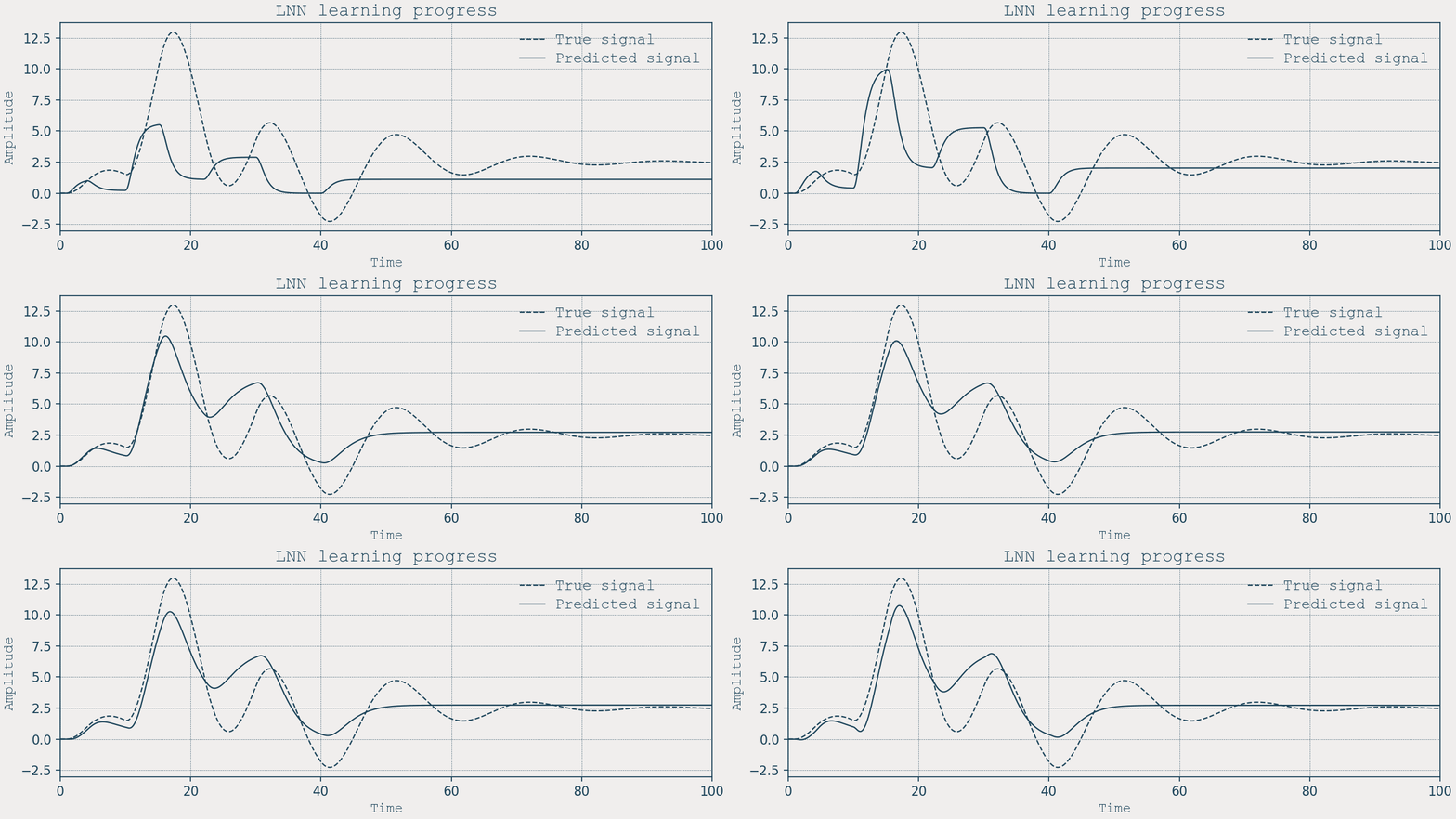
We train with vanilla SGD on both edge weights and neuron parameters:
for epoch in range(2000):
    stats = net.train_step(target=position, lr_w=1e-4, lr_p=1e-3)
    if epoch % 20 == 0:
        print(f"Epoch {epoch:3d} | loss ~ {stats['loss']:.6f}")

Extrapolation capabilities
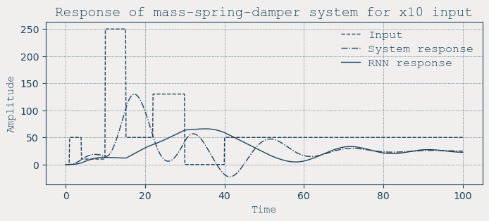
We can probe extrapolation directly: take the training input and scale it ×10, then see if the model still tracks.

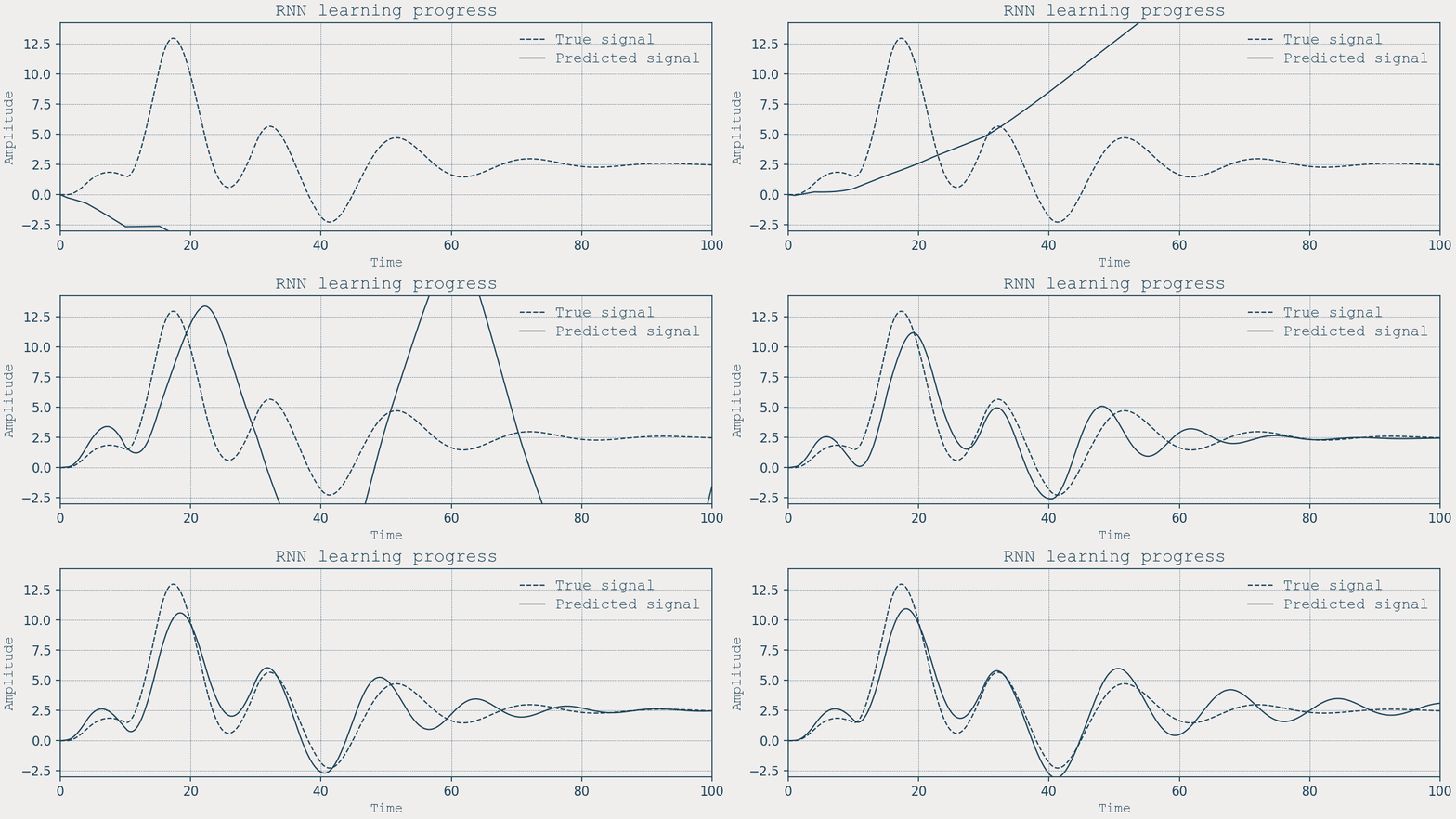
A quasi-fair RNN baseline
To compare, here’s a standard two-layer nn.RNN with a not very similar footprint:
- Input: \([x, \dot{x}, u]\)
- Hidden: 100 units × 2 layers
- Output: \([\dot{x}, \ddot{x}]\) (we predict derivatives and integrate with Euler)
We train on 20-step sequences using MSE on \(d\mathbf{s}/dt\), then simulate closed-loop on the full horizon, including the same ×10 input scale test.
class RNNDynamicsModel(nn.Module):
    def __init__(self, state_dim=2, input_dim=1, hidden_dim=100):
        super().__init__()
        self.rnn1 = nn.RNN(input_size=state_dim+input_dim, hidden_size=hidden_dim, batch_first=True)
        self.rnn2 = nn.RNN(input_size=hidden_dim,        hidden_size=hidden_dim, batch_first=True)
        self.fc   = nn.Linear(hidden_dim, state_dim)  # predicts d[state]/dt

    def forward(self, s_seq, u_seq):
        x = torch.cat([s_seq, u_seq], dim=-1)
        h1,_ = self.rnn1(x)
        h2,_ = self.rnn2(h1)
        return self.fc(h2)


A few notes on parity and scale:
- Parameter count.
– LNN: ~36 trainables (≈15 edges + 7 neurons × 3 params).
– RNN: ~31k trainables (two 100-unit RNN layers + a small head). - Stability constraints. LNN enforces \(\tau,\zeta>0\). The RNN has no built-in stability prior; closed-loop rollout can drift.
What differs and why it matters
1. Where the memory lives
- LNN: memory is physical (time constants in TFs). You never unroll, you simulate LTI blocks once per neuron.
- RNN: memory is parametric (hidden state). You must unroll through time and backpropagate through that unroll (or train on short windows and hope it generalizes).
- LNN: gradients flow through transfer-function algebra. The key objects are \(H_j, G_j\) and \(\partial H_j/\partial\theta\). No vanishing/exploding from long unrolls, the temporal convolution is handled by the TF itself (as promised last time).
- RNN: classic BPTT through many steps. Mitigations (gating, normalization, careful LR) help, but the mechanism remains recursive.
- LNN: linear dynamics + simple nonlinearity (if you insert one) → predictable scaling (our ×10 test).
- RNN: excellent at interpolation; extrapolation depends on how the hidden state happened to encode scale during training.
- LNN: parameters \((k,\tau,\zeta)\) are interpretable time/gain constants per neuron; learned edge weights show the effective signal pathways.
- RNN: internal state is opaque.
Side-by-side summary
| Aspect | Laplace Neural Network | RNN (vanilla, 2×100) |
|---|---|---|
| Trainables (this setup) | ~36 | ~31,000 |
| Memory mechanism | Time constants in TFs | Hidden state |
| Gradient path | Through TF compositions (no BPTT) | BPTT through time |
| Stability prior | \(\tau,\zeta>0\) (enforced) | None (learned implicitly) |
| Generalization to ×10 input | Linear w.r.t. TF | Non-guaranteed; can drift |
| Interpretability | High | Low |
Where to go next
- Insert the \(\delta\)ReLU (or any static nonlinearity) before each LTI block to get a Hammerstein-style LNN and repeat the experiment and watch the residual shrink on non-linear plants.
- Replace first-order \(H_j\) with second-order blocks for oscillatory modes.