How to model the world? Introduction to Laplace Neuron

A growing number of researchers in the AI field are convinced that Large Language Models (LLMs) might be all we need to reach Artificial General Intelligence (AGI). Some even go so far as to claim that LLMs are already building internal world models. And they might not be entirely wrong, if we reduce the idea of a "world model" to nothing more than next-token probability, derived from patterns in an abstract n-dimensional function space.

But what if we take that term more seriously? What if a world model should actually represent... well, a world?

And what is a world, anyway? How could anyone hope to represent it in the clean, formal language of mathematics? We may never fully grasp the whole of what a world is, not with its immense complexity and the intricate network of causal relationships between all kinds of entities.

Still, for the sake of this post, let me propose one particular perspective: let’s think of the world as a hierarchy of dynamical systems. In fact, let’s go further and say the world is the dynamical system that contains all other dynamical systems, except itself.

So the question becomes: how do we model such a thing? Could well-known architectures like Transformers or Recurrent Neural Networks (RNNs) be enough to manage the job? Or do we need an entirely new paradigm?

Dynamical system as dynamical system's model

"A map is not the territory it represents, but, if correct, it has a similar structure to the territory, which accounts for its usefulness." — Alfred Korzybski

What if the map was made of the same stuff as the territory? That may sound paradoxical, or even absurd because a model that fully replicates the system becomes that system. Models are simplified by design. That’s the point.

Still, there is something interesting about the idea of what kind of simplification we choose.

Take the brain. It clearly doesn't hold a full copy of the world, but it contains a highly effective model of it. One possible reason is that it shares a deep structural property with the world itself. The brain is a dynamical system. A nonlinear dynamical system, nonetheless.

Biological neurons are not just static functions that map inputs to outputs. They have internal state. They evolve over time. They integrate signals, respond with delays, build up energy, decay, reset, and interact through feedback loops. They don’t just compute outputs from inputs, they "behave".

Artificial neurons, on the other hand, are fundamentally static. Their output is a direct function of their input at a single point in time. There is no inner process. No memory. No evolution, unless explicitly added by architectural tricks like recurrence.

That might be one of the reasons biological systems are so good at modeling the world. Not because they are more powerful in a raw computational sense, but because they are structurally closer to the kind of thing they are modeling.

In other words, the brain works as a simplified model of the world not just because of what it abstracts away, but because of what it keeps: its dynamic nature.

So what if we used that idea more directly? What if we didn’t rely on stacks of static neurons to simulate motion, feedback, and temporal structure from the outside?

What if we started with a dynamical system as the fundamental building block?

Not because we want to recreate the world in full detail, but because a process might be the best way to model another process.

Laplace Neuron

To make an artificial neuron that is dynamical in its essence, I’ll use a well-known concept from engineering called the transfer function. There are different ways to think about what a transfer function is, but the most intuitive one is that the transfer functions describe how the linear, time-invariant system responds to the input signal or excitation. Basically, how a system reacts to being poked.

Let's break down what "linear" and "time-invariant" actually mean: * Linear means the system obeys the principle of superposition: if you input a sum of signals, the output is the sum of the individual outputs, and scaling the input scales the output by the same factor * Time-invariant means the system’s behavior does not change over time: if you delay the input by some amount, the output is simply delayed by the same amount, with no other changes.

Transfer functions are a way to describe how systems behave over time. But instead of writing out full differential equations, we move into a different space, the \(s\) domain, also called the Laplace domain.

In the \(s\) domain, time becomes complex frequency. Derivatives turn into multiplications. What was complex and messy in the time domain becomes simpler, more compact. That’s why engineers and control theorists like it. And more importantly for us, it gives us a language to talk about dynamics, about how inputs change into outputs, not instantly, but through some process that unfolds in time.

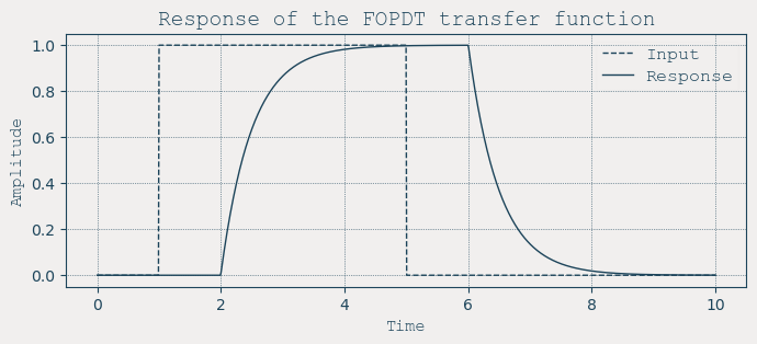
To keep it simple, I’ll use a well-known transfer function called First Order Plus Dead Time (FOPDT). It looks like this:

H(s) = \frac{Y(s)}{U(s)} = e^{-\theta s} \cdot \frac{K}{\tau s + 1}

This may look abstract, but it actually describes something very familiar: a system that waits a bit, then starts reacting gradually.

Let’s break it down:

\(Y(s)\) is the output of the system in the \(s\) domain
\(U(s)\) is the input signal in the \(s\) domain
\(K\) is the gain — it tells you how much output you get per unit of input
\(\tau\) is the time constant — how fast the system reacts. A small \(\tau\) means a quick response, large \(\tau\) means slower response
\(\theta\) is the dead time — the delay before the system even starts responding
\(s\) is the Laplace variable, \(s = \sigma + j \omega\), combining exponential decay and oscillation

So what does this function mean in practice?

Imagine you flip a switch. The system doesn’t respond right away, that’s the dead time \(\theta\). After that, the output starts rising, not instantly, but with a certain smoothness. That smoothness comes from \(\tau\). And how high the output goes, that depends on \(K\).

With just these three parameters, gain, time constant, and dead time, you can model a huge number of simple real-world processes. From heating up water to the way your muscles respond to a nerve signal.

And this is the core idea I want to carry forward.

Because if we want to model a system like the brain, or even just a single neuron, we need something that can describe change. Not just inputs and outputs, but the path between them. The delay, the buildup, the decay.

Building up complexity

Since our current transfer function is linear, it’s time to introduce some nonlinearity to better resemble the kind of behavior we observe in biological neurons. Biological neurons are often associated with the idea of thresholds. There is a certain level of stimulation a neuron must receive before it "fires", a critical point it must cross before it starts propagating the signal forward. This concept is crucial if we want our Laplace Neuron to start behaving more like its biological counterpart.

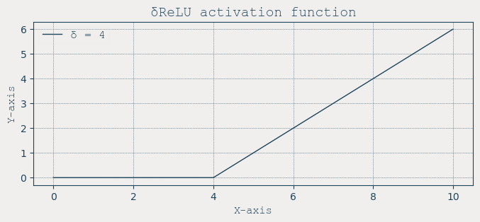
Let’s introduce what I call the \(\delta\)ReLU, defined by the following equation:

\delta \mathrm{ReLU}(x) = \begin{cases} x & \text{if } x>\delta \\ 0 & \text{otherwise} \end{cases}

The \(\delta\)ReLU is just a generalization on the familiar Rectified Linear Unit (ReLU). It works in much the same way: if the input is below a certain value, the output is zero, if the input crosses that value, it passes through linearly. The difference here is the parameter \(\delta\), which explicitly defines the firing threshold. This is the point where the neuron switches from silence to activity. Below \(\delta\), the neuron remains silent. Once the input breaches this threshold, the neuron becomes active, and the signal flows through.

Why not just use regular ReLU you may ask?

Suppose we are trying to model a constrained physical system, one that only operates in the positive domain. The regular ReLU won’t help us much here. It activates at zero, but that’s not a meaningful boundary in many real-world systems. \(\delta\)ReLU lets us set a threshold that actually corresponds to some meaningful constraint in the system we’re modeling. The same logic applies to biased systems, like biological neurons that fire at approximately \(-55 mV\). In that case, we’d simply set \(\delta = -55\).

Now, what exactly causes a Laplace Neuron to fire?

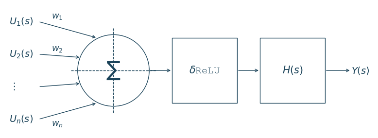
Just like in the classic model of an artificial neuron, the Laplace Neuron gets excited by the weighted sum of all the other Laplace Neurons connected to it. Every input contributes its part. The sum is calculated, and if it crosses the threshold \(\delta\), the neuron responds.

So with this, we have a structure that starts to look and behave more like a real neuron. It has dynamics through the transfer function. It has a threshold through \(\delta\)ReLU. And it interacts with other neurons through weighted connections.

Now it's time to bring it all together, wrap everything into a single equation that captures the principle of Laplace Neuron.

Mathematical definition of the Laplace Neuron

Y(s) = \mathcal{L} \left\{ \delta\mathrm{ReLU} \left[ \mathcal{L}^{-1} \left( \sum_{j=1}^{n} w_j \, U_j(s) \right) \right] \right\} \cdot e^{-\theta s} \cdot \frac{K}{\tau s + 1}

\(Y(s)\) is the output in the Laplace domain
\(\delta\mathrm{ReLU}\) is activation function
\(\sum_{j=1}^{n} {w_j}{U_j(s)}\) is weighted sum of inputs
\(e^{-\theta s}\frac{K}{\tau s+1}\) is first order plus dead time transfer function
\(\mathcal{L} \left {f}(s) \right] = \int_{0}^{\infty} f(t)e^{-st} \, dt \) is the Laplace transform
\(\mathcal{L}^{-1}\) is the inverse of the Laplace transform

Or, in a more intuitive time-domain form:

y(t) = \mathcal{L}^{-1} \left\{ \mathcal{L} \left[ \delta \mathrm{ReLU} \left( \sum_{j=1}^{n} w_j \, u_j(t) \right) \right] \cdot e^{-\theta s} \cdot \frac{K}{\tau s + 1} \right\}

We can also rewrite the transfer function in the time domain and represent it as a state-space model as follows:

\dot{x}(t) = A\cdot x(t) + B\cdot \delta\mathrm{ReLU}[u(t - \theta)]

y(t) = C\cdot x(t)

where:

\(x(t)\) is state vector
\(u(t - \theta)\) is delayed input vector
\(y(t)\) is output vector
\(A,B,C\) are state-space matrices defined by transfer function

The state-space representation might look oddly familiar. Once we discretize it, it almost becomes the vanilla formulation of a Recurrent Neural Network (RNN).

Surprised? You shouldn’t be.

At its core, the RNN is just a system that loops its own state through time. It takes an input, blends it with memory, and hands itself back the result, over and over again. In other words, it is a dynamical system.

But here's the twist: what we’ve done here is not just rediscover the RNN. We've reinterpreted it through the lens of continuous and constrained physical systems. The Laplace Neuron doesn’t just mimic the RNN update rule, it is one, but with a structure that maps more naturally to real-world dynamics.

So maybe the architectures we've had all along weren't completely off. Maybe they just needed to be seen from the right angle.

In the next post, I’ll dive into the differences between the Laplace Neuron and the classic RNN, and explore why the Laplace Neuron might hold a serious advantage when it comes to the learning process, by solving the vanishing and exploding gradient problem.

Stay tuned. It gets interesting.

Related work

Hammerstein/Wiener models: Static nonlinearity followed by LTI cascades. Laplace neuron is Hammerstein type of model (nonlinearity is on the input).
Continuous-time neural models: Neural ODEs; Liquid Time-constant Networks.
State-space models (SSMs): S4/S4D and successors (long-range sequence modeling via learned linear dynamics). Laplace neuron is a first-order, interpretable variant with explicit \(K\), \(\tau\) and \(\theta\).